Operating Systems(OS)

How an operating system can maximise the use of computer resources

• When a computer is first switched on, the basic input/output system (BIOS) – which is often stored on the ROM chip – starts off a bootstrap program.

• The bootstrap program loads part of the operating system into main memory (RAM) from the hard disk/SSD and initiates the start-up procedures.

• This process is less obvious on tablets and mobile phones – they also use RAM, but their main internal memory is supplied by flash memory; this explains why the start-up of tablets and mobile phones is almost instantaneous.

• The flash memory is split into two parts.

  1. The part where the OS resides.
  2. The part where the apps (and associated data) are stored.

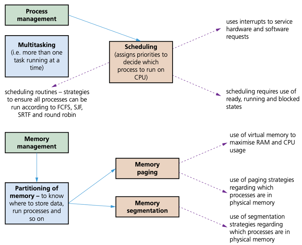
• One operating system task is to maximise the utilisation of computer resources.

• Resource management can be split into three areas

  1. the CPU
  2. memory
  3. the input/output (I/O) system.

• Resource management of the CPU involves the concept of scheduling to allow for better utilisation of CPU time and resources.

• Regarding input/output operations, the operating system will need to deal with

  • any I/O operation which has been initiated by the computer user
  • any I/O operation which occurs while software is being run and resources, such as printers or disk drives, are requested.

The kernel

• The kernel is part of the operating system.
• It is the central component responsible for communication between hardware, software and memory.
• It is responsible for process management, device management, memory management, interrupt handling and input/output file communications

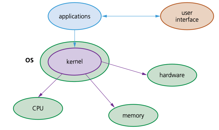
Hide the complexities

• One of the most important tasks of an operating system is to hide the complexities of the hardware from the users.
• This can be done by
  • using GUI interfaces rather than CLI
  • using device drivers (which simplifies the complexity of hardware interfaces)
  • simplifying the saving and retrieving of data from memory and storage devices
  • carrying out background utilities, such as virus scanning which the user can ‘leave to its own devices’.

Multitasking

• Multitasking allows computers to carry out more than one task (known as a process) at a time. (A process is a program that has started to be executed.)
• Each of these processes will share common hardware resources.
• To ensure multitasking operates correctly (for example, making sure processes do not clash), scheduling is used to decide which processes should be carried out.
• Scheduling is considered in more depth in the next section.
• Multitasking ensures the best use of computer resources by monitoring the state of each process.
• It should give the appearance that many processes are being carried out at the same time.
• In fact, the kernel overlaps the execution of each process based on scheduling algorithms.
• There are two types of multitasking operating systems
  1. preemptive (processes are pre-empted after each time quantum)
  2. non-preemptive (processes are pre-empted after a fixed time interval).

Preemptive	Non-preemptive
resources are allocated to a process for alimited time	once the resources are allocated to aprocess, the process retains them untilit has completed itsburst timeor theprocess has switched to a waiting state
the process can be interrupted while it isrunning	the process cannot be interrupted whilerunning; it must first finish or switch to awaiting state
high priority processes arriving in theready queue on a frequent basis can meanthere is a risk that low priority processesmay bestarvedof resources	if a process with a long burst time isrunning in the CPU, there is a risk thatanother process with a shorter burst timemay be starved of resources
this is a more flexible form of scheduling	this is a more rigid form of scheduling

Low level scheduling

• Low level scheduling decides which process should next get the use of CPU time (in other words, following an OS call, which of the processes in the ready state can now be put into a running state based on their priorities).
• Its objectives are to maximise the system throughput, ensure response time is acceptable and ensure that the system remains stable at all times (has consistent behaviour in its delivery).
• For example, low level scheduling resolves situations in which there are conflicts between two processes requiring the same resource.
• Suppose two apps need to use a printer; the scheduler will use interrupts, buffers and queues to ensure only one process gets printer access – but it also ensures that the other process gets a share of the required resources.

Process scheduler

• Process priority depends on

  • its category
  • whether the process is CPU-bound
  • resource requirements
  • the turnaround time, waiting time and response time for the process
  • whether the process can be interrupted during running.

• Once a task/process has been given a priority, it can still be affected by

  • the deadline for the completion of the process
  • how much CPU time is needed when running the process
  • the wait time and CPU time
  • the memory requirements of the process.

Process states

• A process control block (PCB) is a data structure which contains all of the data needed for a process to run; this can be created in memory when data needs to be received during execution time.
• The PCB will store
  • current process state (ready, running or blocked)
  • process privileges (such as which resources it is allowed to access)
  • register values (PC, MAR, MDR and ACC)
  • process priority and any scheduling information
  • the amount of CPU time the process will need to complete
  • a process ID which allows it to be uniquely identified.
• A process state refers to the following three possible conditions
  1. running
  2. ready
  3. blocked

The link between these three conditions

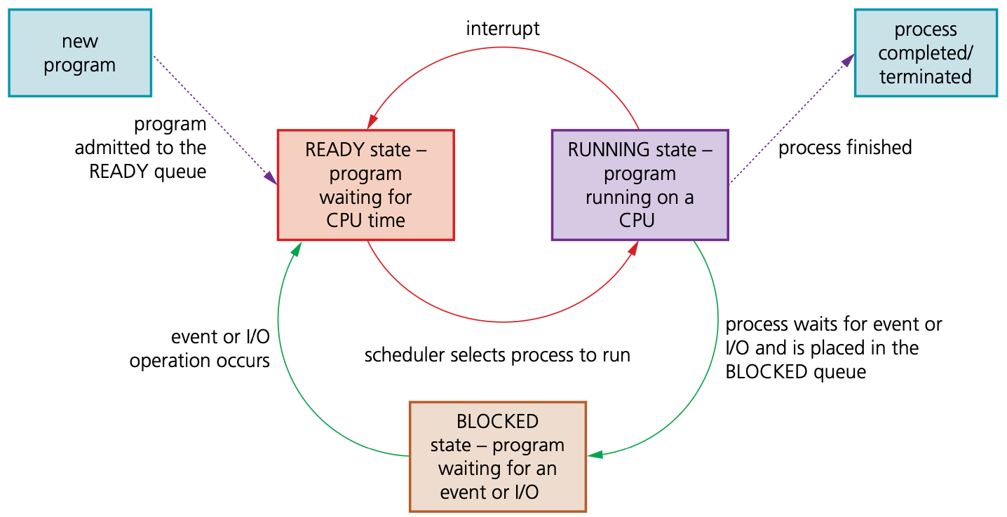
Some of the conditions when changing from one process state to another.

Process states	Conditions
running state→ready state	a program is executed during its time slice; when the timeslice is completed an interrupt occurs and the program ismoved to the READY queue
ready state→running state	a process’s turn to use the processor; the OS schedulerallocates CPU time to the process so that it can be executed
running state→blocked state	the process needs to carry out an I/O operation; the OSscheduler places the process into the BLOCKED queue
blocked state→ready state	the process is waiting for an I/O resource; an I/Ooperation is ready to be completed by the process

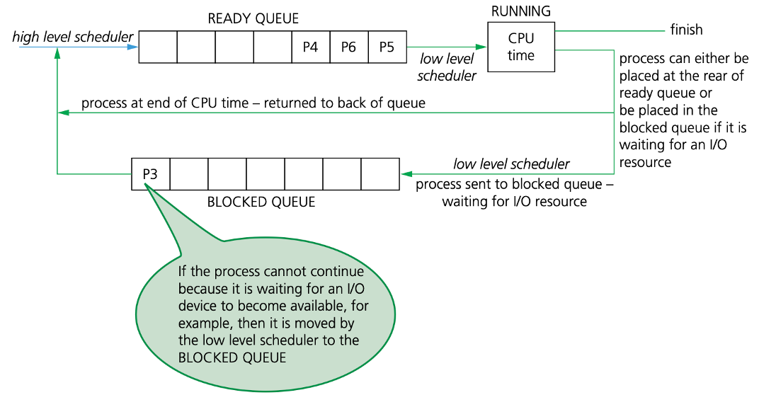
• To investigate the concept of a READY QUEUE and a BLOCKED QUEUE a little further, we will consider what happens during a round robin process, in which each of the processes have the same priority.
• Supposing two processes, P1 and P2, have completed. The current status is shown in Figure.

Scheduling routine algorithms

• We will consider four examples of scheduling routines

  1. first come first served scheduling (FCFS)
  2. shortest job first scheduling (SJF)
  3. shortest remaining time first scheduling (SRTF)
  4. round robin

• These are some of the most common strategies used by schedulers to ensure the whole system is running efficiently and in a stable condition at all times.

• It is important to consider how we manage the ready queue to minimise the waiting time for a process to be processed by the CPU.

First come first served scheduling (FCFS)

• This is similar to the concept of a queue structure which uses the first in first out (FIFO) principle.
• The data added to a queue first is the data that leaves the queue first.
• Suppose we have four processes, P1, P2, P3 and P4, which have burst times of 23ms, 4ms, 9ms and 3ms respectively.
• The ready queue will be

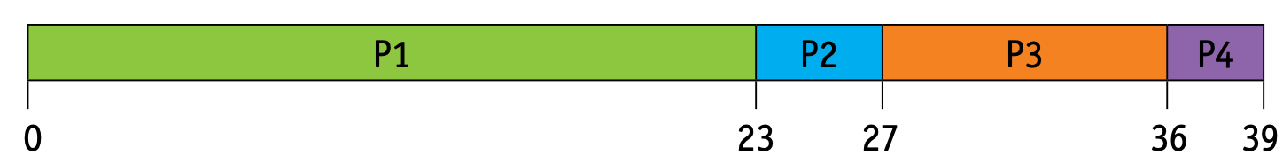
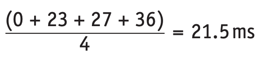
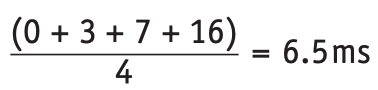
• This will give the average waiting time for a process as:

Shortest job first scheduling (SJF) and shortest remaining time first scheduling (SRTF)

• These are the best approaches to minimise the process waiting times.
• SJF is non-preemptive and SRTF is preemptive.
• The burst time of a process should be known in advance; although this is not always possible.
• We will consider the same four processes and burst times as the above example (P1 = 23ms, P2 = 4ms, P3 = 9ms, P4 = 3ms).
• With SJF, the process requiring the least CPU time is executed first.
• P4 will be first, then P2, P3 and P1. The ready queue will be

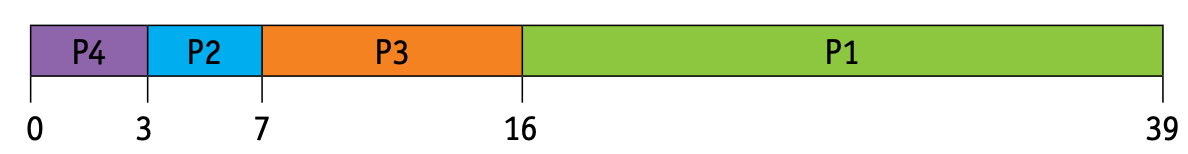
• The average waiting time for a process will be

• With SRTF, the processes are placed in the ready queue as they arrive; but when a process with a shorter burst time arrives, the existing process is removed (pre-empted) from execution.
• The shorter process is then executed first.
• Let us consider the same four processes, including their arrival times.
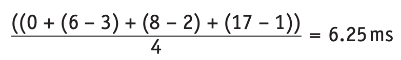
• The ready queue will be

The average waiting time for a process will be

Round robin

• A fixed time slice is given to each process; this is known as a quantum.
• Once a process is executed during its time slice, it is removed and placed in the blocked queue; then another process from the ready queue is executed in its own time slice.
• Context switching is used to save the state of the pre-empted processes.
• The ready queue is worked out by giving each process its time slice in the correct order (if a process completes before the end of its time slice, then the next process is brought into the ready queue for its time slice).
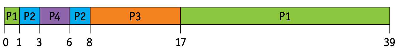
• Thus, for the same four processes, P1–P4, we get this ready queue

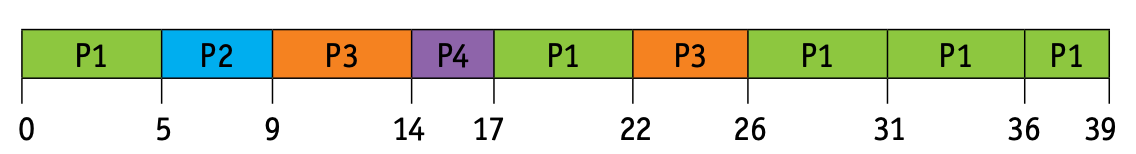
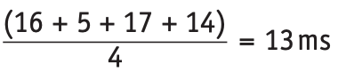
• The average waiting time for a process is calculated as follows:
• P1: (39 – 23) = 16ms
• P2: (9 – 4) = 5ms
• P3: (26 – 9) = 17ms
• P4: (17 – 3) = 14ms
• Thus, average waiting time

Scheduling routine algorithms

• We will consider four examples of scheduling routines

  1. first come first served scheduling (FCFS)
  2. shortest job first scheduling (SJF)
  3. shortest remaining time first scheduling (SRTF)
  4. round robin

• the average waiting times for the four scheduling routines

FCFS	21.5 ms
SJF	6.5ms
SRTF	6.25 ms
Round robin	13.0ms

Interrupt handling and OS kernels

• The CPU will check for interrupt signals.

• The system will enter the kernel mode if any of the following type of interrupt signals are sent:

  • Device interrupt (for example, printer out of paper, device not present, and so on).
  • Exceptions (for example, instruction faults such as division by zero, unidentified op code, stack fault, and so on).
  • Traps/software interrupt (for example, process requesting a resource such as a disk drive).

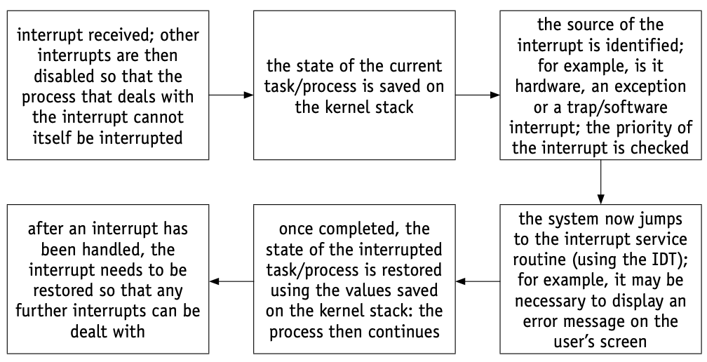
• When an interrupt is received, the kernel will consult the interrupt dispatch table (IDT) – this table links a device description with the appropriate interrupt routine.

• IDT will supply the address of the low level routine to handle the interrupt event received.

• The kernel will save the state of the interrupt process on the kernel stack and the process state will be restored once the interrupting task is serviced.

• Interrupts will be prioritised using interrupt priority levels (IPL) (numbered 0 to 31).

• A process is suspended only if its interrupt priority level is greater than that of the current task.

Memory management

• As with the storage of data on a hard disk, processes carried out by the CPU may also become fragmented.
• To overcome this problem, memory management will determine which processes should be in main memory and where they should be stored (this is called optimisation); in other words, it will determine how memory is allocated when a number of processes are competing with each other.
• When a process starts up, it is allocated memory; when it is completed, the OS deallocates memory space.

Single (contiguous) allocation

• With this method, all of the memory is made available to a single application.
• This leads to inefficient use of main memory.

Paged memory/paging

• In paging, the memory is split up into partitions (blocks) of a fixed size.

• The partitions are not necessarily contiguous. The physical memory and logical memory are divided up into the same fixed-size memory blocks.

• Physical memory blocks are known as frames and fixed-size logical memory blocks are known as pages.

• A program is allocated a number of pages that is usually just larger than what is actually needed.

• When a process is executed, process pages from logical memory are loaded into frames in physical memory.

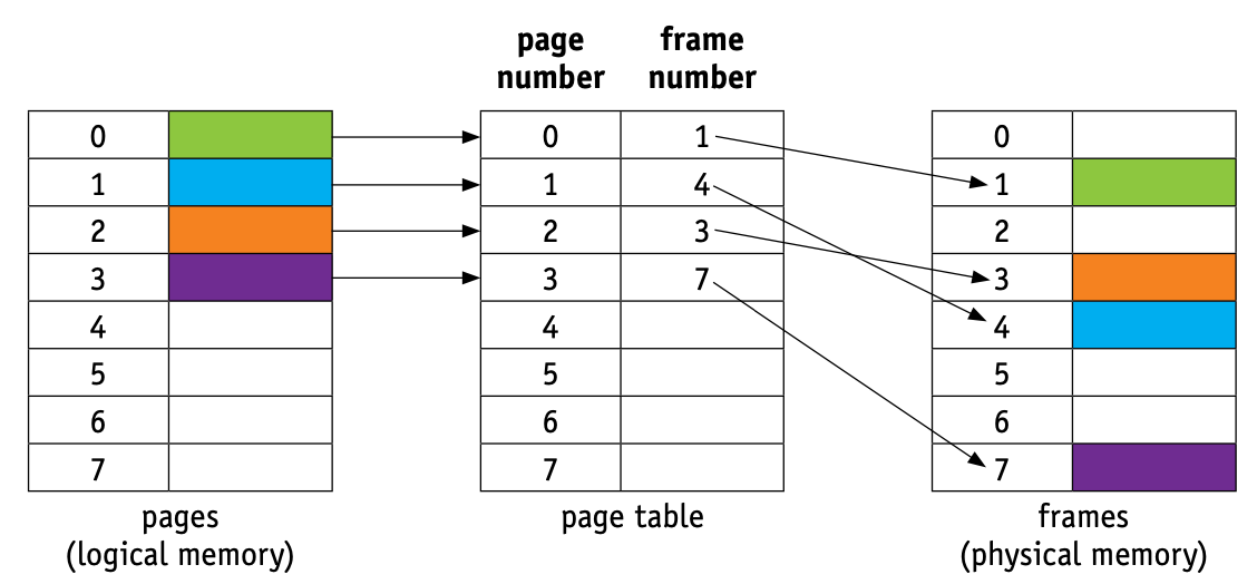
• A page table is used; it uses page number as the index.

• Each process has its own separate page table that maps logical addresses to physical addresses.

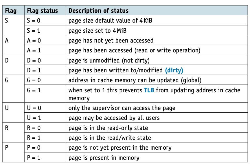
• The page table will show page number, flag status, page frame address, and the time of entry (for example, in the form 08:25:55:08).

• The time of entry is important when considering page replacement algorithms.

• Some of the page table status flags are shown in Table below.

• The following diagram only shows page number and frame number (we will assume status flags have been set and entry time entered).
• Each entry in a page table points to a physical address that is then mapped to a virtual memory address – this is formed from offset in page directory + offset in page table.

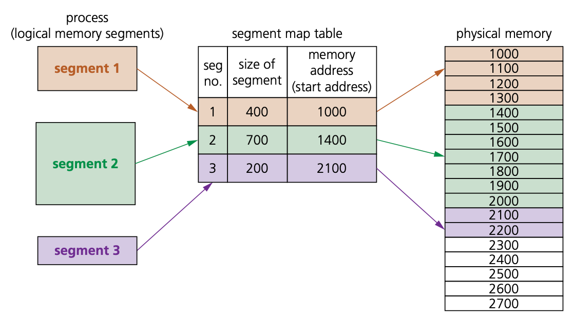
Segmentation/segmented memory

• In segmented memory, logical address space is broken up into variable-size memory blocks/partitions called segments.
• Each segment has a name and size. For execution to take place, segments from logical memory are loaded into physical memory.
• The address is specified by the user which contains the segment name and offset value.
• The segments are numbered (called segment numbers) rather than using a name and this segment number is used as the index in a segment map table. The offset value decides the size of the segment:

address of segment in physical memory space = segment number + offset value

• The segment map table in Figure contains the segment number, segment size and the start address in physical memory.
• Note that the segments in logical memory do not need to be contiguous, but once loaded into physical memory, each segment will become a contiguous block of memory.
• Segmentation memory management works in a similar way to paging, but the segments are variable sized memory blocks rather than all the same fixed size.

Summary of the differences between paging and segmentation

Paging	Segmentation
a page is a fixed-size block of memory	a segment is a variable-size block ofmemory
since the block size is fixed, it is possiblethat all blocks may not be fully used – thiscan lead to internal fragmentation	because memory blocks are a variable size,this reduces risk of internal fragmentationbut increases the risk of externalfragmentation
the user provides a single value – thismeans that the hardware decides theactual page size	the user will supply the address in twovalues (the segment number and thesegment size)
a page table maps logical addresses tophysical addresses (this contains the baseaddress of each page stored in frames inphysical memory space)	segmentation uses a segment map tablecontaining segment number + offset(segment size); it maps logical addresses tophysical addresses
the process of paging is essentiallyinvisible to the user/programmer	segmentation is essentially a visibleprocess to a user/programmer
procedures and any associated data cannotbe separated when using paging	procedures and any associated data can beseparated when using segmentation
paging consists of static linking anddynamic loading	segmentation consists of dynamic linkingand dynamic loading
pages are usually smaller than segments	pages are usually smaller than segments

Virtual memory

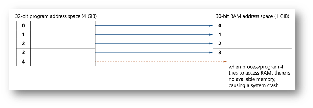
• One of the problems encountered with memory management is a situation in which processes run out of RAM main memory.

• If the amount of available RAM is exceeded due to multiple processes running, it is possible to corrupt the data used in some of the programs being run.

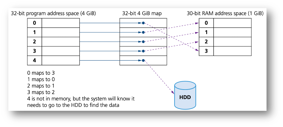
• This can be solved by separately mapping each program’s memory space to RAM and utilising the hard disk drive (or SSD) if we need more memory. This is the basis behind virtual memory.

• Essentially, RAM is the physical memory and virtual memory is RAM + swap space on the hard disk (or SSD).

• Virtual memory is usually implemented using in demand paging (segmentation can be used but is more difficult to manage).

• To execute a program, pages are loaded into memory from HDD (or SSD) whenever required.

• We can show the differences between paging without virtual memory and paging using virtual memory in two simple diagrams

Without virtual management

With virtual management

• The main benefits of virtual memory are

  • programs can be larger than physical memory and can still be executed
  • it leads to more efficient multi-programming with less I/O loading and swapping programs into and out of memory
  • there is no need to waste memory with data that is not being used (for example, during error handling)
  • it eliminates external fragmentation/reduces internal fragmentation
  • it removes the need to buy and install more expensive RAM memory.

• The main drawback when using HDD is that, as main memory fills, more and more data/pages need to be swapped in and out of virtual memory.

• This leads to a high rate of hard disk read/write head movements; this is known as disk thrashing.

• If more time is spent on moving pages in and out of memory than actually doing any processing, then the processing speed of the computer will be reduced.

• A point can be reached when the execution of a process comes to a halt since the system is so busy paging in and out of memory; this is known as the thrash point.

• Due to large numbers of head movements, this can also lead to premature failure of a hard disk drive.

• Thrashing can be reduced by installing more RAM, reducing the number of programs running at a time, or reducing the size of the swap file.

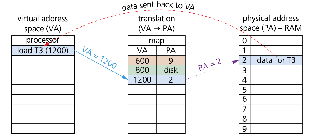
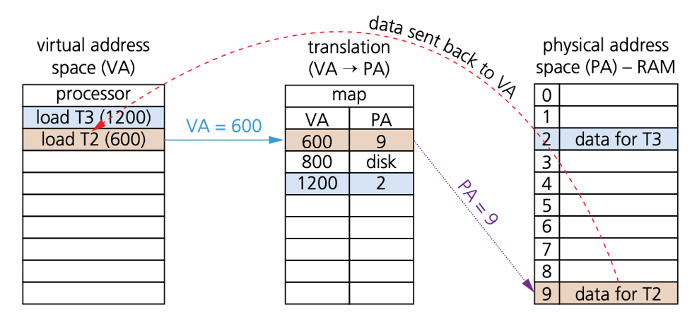
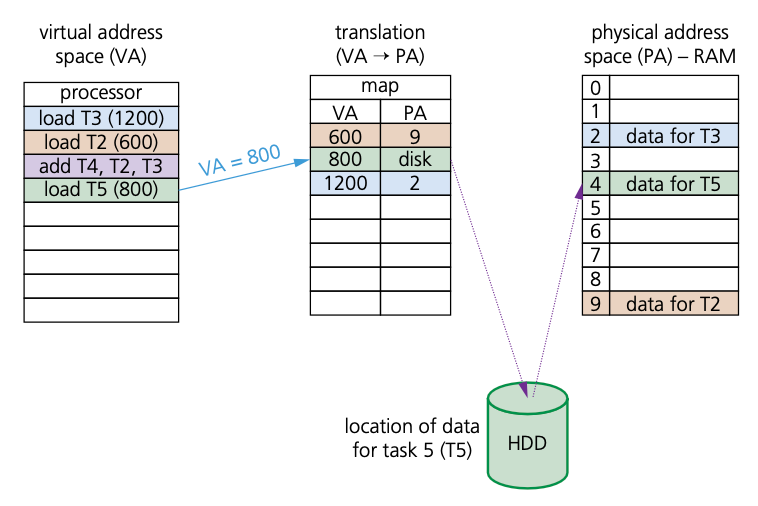
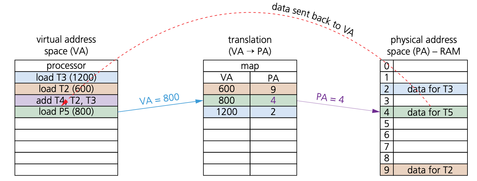
How do programs/processes access data when using virtual memory

• Virtual memory is used in a more general sense to manage memory using paging:
  • The program executes the load process with a virtual address (VA).
  • The computer translates the address to a physical address (PA) in memory.
  • If PA is not in memory, the OS loads it from HDD.
  • The computer then reads RAM using PA and returns the data to the program.

Page replacement

• Page replacement occurs when a requested page is not in memory (P flag = 0).
• When paging in/out from memory, it is necessary to consider how the computer can decide which page(s) to replace to allow the requested page to be loaded.
• When a new page is requested but is not in memory, a page fault occurs and the OS replaces one of the existing pages with the new page(s).
• How to decide which page to replace is done in a number of different ways, but all methods have the same goal of minimising the number of page faults.
• A page fault is a type of interrupt (it is not an error condition) raised by hardware.
• When a running program accesses a page that is mapped into virtual memory address space, but not yet loaded into physical memory, then the hardware needs to raise this page fault interrupt.

Page replacement algorithms

First in first out (FIFO)

• When using first in first out (FIFO), the OS keeps track of all pages in memory using a queue structure.
• The oldest page is at the front of the queue and is the first to be removed when a new page needs to be added.
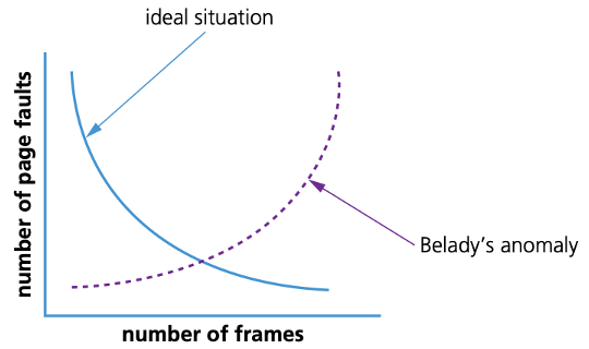
• FIFO algorithms do not consider page usage when replacing pages: a page may be replaced simply because it arrived earlier than another page.
• It suffers from what is known as Belady’s anomaly, a situation in which it is possible to have more page faults when increasing the number of page frames – this is the reverse of the ideal situation shown by the graph in Figure.

Optimal page replacement (OPR)

• Optimal page replacement looks forward in time to see which frame it can replace in the event of a page fault.
• The algorithm is impossible to implement; at the time of a page fault, the OS has no way of knowing when each of the pages will be replaced next.
• It tends to get used for comparison studies – but it has the advantage that it is free of Belady’s anomaly and has the fewest page faults.

Least recently used page replacement (LRU)

• With least recently used page replacement (LRU), the page which has not been used for the longest time is replaced.
• To implement this method, it is necessary to maintain a linked list of all pages in memory with the most recently used page at the front and the least recently used page at the rear.

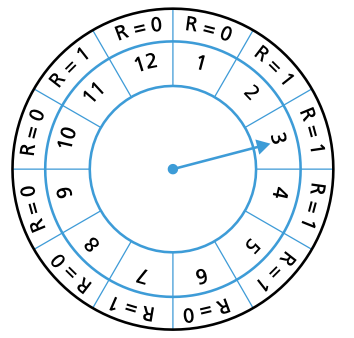
Clock page replacement/second-chance page replacement

• Clock page replacement algorithms use a circular queue structure with a single pointer serving as both head and tail.
• When a page fault occurs, the page pointed to (element 3 in the diagram on the following page) is inspected.
• The action taken next depends on the R-flag status.
• If R = 0, the page is removed and a new page inserted in its place; if R = 1, the next page is looked at and this is repeated until a page where R = 0 is found.

Processor management and memory management

• Processor management decides which processes will be executed and in which order (to maximise resources), whereas memory management will decide where in memory data/programs will be stored and how they will be stored.
• Although quite different, both are essential to the efficient and stable running of any computer system.